Gradient Boosted Decision Trees
I got to know the series of Gradient Boosted Decision Trees (GBDT) at the time for developing classification/regression algorithms for time series data. GBDT algorithms include XGBoost, LightGBM and CatBoost. This article gives a brief explanation of the basic idea of GBDT.
Useful Resources (References)
Questions
When we come to algorithms based on trees, we would like to know some questions of how to construct trees. Specifically, the trees have leaf nodes and splitting nodes. The questions are listed below:
- How to choose the proper features and the value of the features for constructing a splitting nodes?
- When to stop split the node and obtain the leaf node?
- How to combine the results of different trees or what are the relationships between different trees?
- How to constrain the size of trees?
In the following sections, these questions will be answered.
GBDT trees for regression
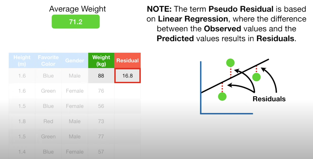
Let’s start with building trees for regression. Given an example of predicting weights from height, favorite color, and gender shown in the figure below:

General ideas
Initially, the first tree (stump) is created by averaging all the weights. It is used as the first decision tree. The difference between the ground truth and the predicted value is called residual.
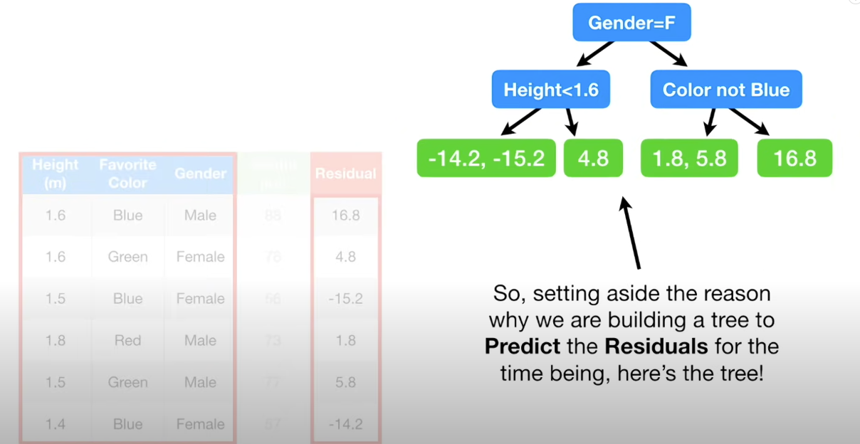
Next, a decision tree for predicting these residuals are created.

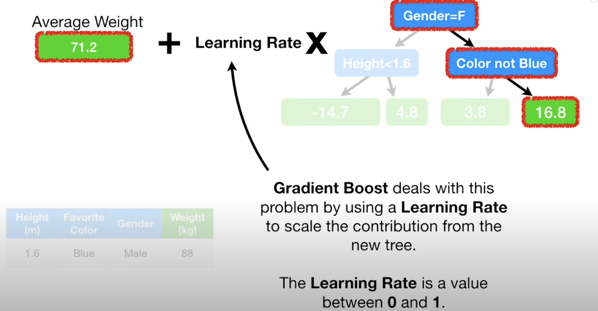
Afterwards, the values of this tree is added to previous tree with a learning rate. This can explain why they are called gradient boosting decision trees. GBDT trees are a bunch of weak learners. In addition, smaller learning rate in right direction can achieve better results with lower variances.

Regression details
How to define the value of leaves

Step 1
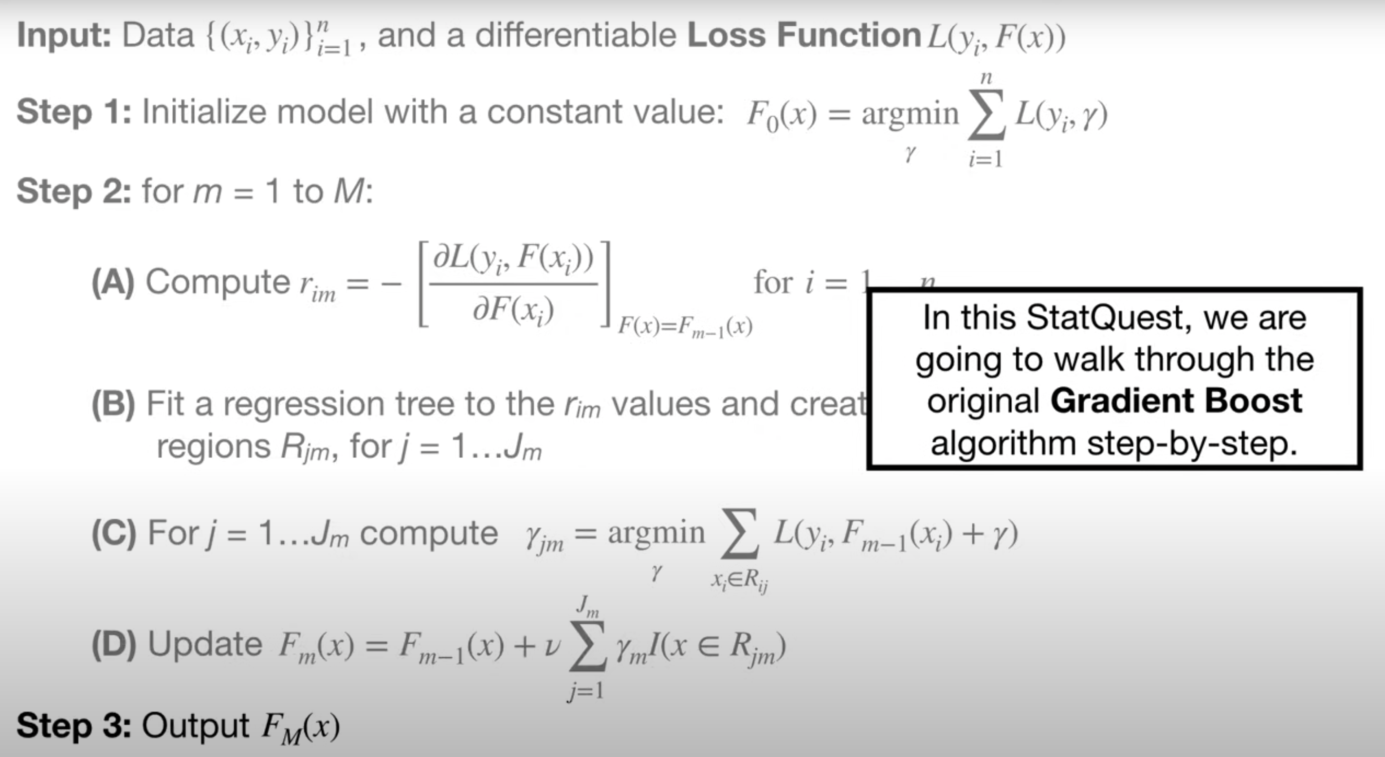
Firstly, initialize the model with a constant value.
\[F_0(x)={argmin}_{r}\sum^n_{i=1}L(y_i, \gamma)\]where (y_i) represents the observed value, (\gamma) represents the leaf value. It can be seen that the leaf value is simple the averaged value of all samples.
Step 2
In the second step, the loss function and its gradient are computed for the pseudo residuals and terminal regions (can be regard as the leaf values).
The loss function is defined by the mean square error,
\[L(y_i, F(x_i)) = (y_i - F(x_i))^2\]where (F(x_i)) is the prediction values from the last tree, (i) represents the index of the training samples. Clearly, the value of the loss function is the (pseudo) residual . Afterwards, different samples are split to different branches, the terminal region (R_{jm}) is found by these sorted pseudo residuals. (j) represents the index of the terminal regions, (m) represents the index of the trees. In addition, the parameter (m) is often called iterations in gbdt packages, for example, LightGBM and CatBoost.
After finding the terminal regions, the leaf values are calculated. The leaf values need to minimize the loss function, they are calculated as follows,
\[\gamma_{jm} = argmin_{\gamma}\sum_{x_i \in R_{ij}}L(y_i, F_{m-1}(x_i) + \gamma)\]where (gamma) is the leaf value.
Finally, the new tree is defined as below,
\[F_m(x) = F_{m-1}(x) + \nu \sum_{j=1}^{J_m} \gamma_m I(x \in R_{jm})\]It can be seen that finding the terminal regions is quite time consuming. Under a split value of a specific feature, it needs to iterate all training samples. Therefore, many optimized GBDT algorithms emerge to improve computing efficiency, such as XGBoost, LightGBM, and CatBoost.